
Speed of Sound in Marching Band: A Sound Delay Calculator for the Football Field
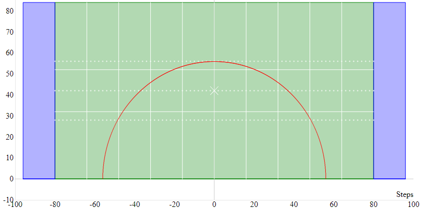
Click the image to check out the easy SoundDelay.com Calculator App!
Understanding how timing actually changes across the field
Marching band and drum corps performers are not simply playing in time with each other. They are also playing in time with physics. On a football field, sound takes time to travel, and that travel time can affect how rhythms are perceived from different locations.
This is the foundation of what I call Cost of Timing. It describes the relationship between tempo, distance, and rhythm when sound moves through space. The farther apart performers are, the greater the delay between when a sound is produced and when that sound is heard by someone somewhere else on the field.
In simple terms, a note played at the back of the field does not arrive at the front at the exact moment it was played. The performer produces the sound first, then the sound travels through the air before reaching the listener. As the distance increases, that delay increases as well.
For marching ensembles, this creates a unique timing challenge. Two performers can technically play at the same tempo while the sound reaching a listener appears slightly misaligned because the sounds traveled different distances. What a performer hears is therefore not always an exact representation of when another performer physically played the note.
The effect becomes more noticeable at faster tempos and over greater distances. A small delay that is barely noticeable at close range can become significant when performers are spread across an entire football field.
Understanding this relationship between tempo, distance, and sound propagation provides a useful framework for analyzing timing problems in marching band and drum corps. Instead of treating every timing discrepancy as a simple performance issue, Cost of Timing considers the physical environment in which the music is being performed.
The field itself becomes part of the timing equation.
Why this matters in marching band and drum corps
There are three practical reasons the concept of Cost of Timing is useful for marching band and drum corps.
First, it helps performers understand how far ahead or behind they may need to play in order for their sound to align with another section. When performers are separated by significant distances, the sound they hear from another performer may arrive later than the moment it was actually produced. Understanding that delay can help performers make more informed timing decisions.
Second, Cost of Timing provides a way to calculate how ensemble timing changes across large field distances. Instead of relying entirely on what the performer hears from their current position, you can consider the distance between performers and estimate how sound travel affects what each person perceives. This creates a more complete picture of ensemble timing across the field.
Third, the concept can be used intentionally when designing drill and music. Spatial timing does not always have to be treated as a problem to overcome. Designers and instructors can consider distance and sound travel when creating musical effects that depend on performers being separated across the field.
Most performers experience timing primarily from their own position. They hear what reaches them and make adjustments based on that perspective. Cost of Timing provides a way to think beyond a single listening position.
By considering tempo, distance, and the speed of sound together, you can estimate how a musical event will be perceived from different locations on the field. This makes it possible to analyze timing from the perspective of the performer, the ensemble, or the audience rather than treating the field as if every sound travels instantaneously.
The result is a more complete way to understand timing in large marching ensembles. Once you account for the physical movement of sound, the field is no longer just the space where the performers stand. It becomes an active part of the timing equation.
The basic idea behind sound delay on the field
Sound travels through air at a predictable speed, which means that for practical outdoor marching applications, we can treat the speed of sound as essentially constant under typical rehearsal conditions. What changes from performer to performer is the distance the sound has to travel.
Consider two performers positioned on opposite sides of a football field. A performer on the back sideline and a performer on the front sideline could play at exactly the same moment, with perfect timing. An audience member will still hear those sounds at slightly different times because the sound from each performer has traveled a different distance.
That difference in arrival time is the Cost of Timing.
The performers may be perfectly synchronized at the moment they produce the sound, but the audience experiences the performance based on when those sounds actually arrive. As the distance between performers and listeners increases, the timing difference becomes more noticeable.
This creates a genuine challenge for large marching ensembles. Performers and instructors cannot always judge timing solely by what they hear because what they hear is affected by where they are standing. A sound coming from across the field has already been delayed by the time it reaches them.
But the same phenomenon can also create creative possibilities.
If designers understand how sound travels across the field, they can intentionally use spatial separation to create musical effects. Different sections can produce sounds at carefully chosen moments and locations, allowing the audience to experience those sounds as staggered arrivals. What might otherwise be treated as a timing problem can become part of the musical design.
The key is understanding the difference between when a sound is produced and when that sound is heard. Those are not always the same moment, especially across the distances involved in marching band and drum corps.
Once that distinction becomes part of the planning process, distance is no longer just a physical measurement on the field. It becomes another variable that can influence ensemble timing, rehearsal technique, and musical design.
Step sizes and field measurement system
Marching band drill is often built on standardized step sizes:
Horizontal step size is 22.5 inches
Vertical step size is approximately 22.857 inches
The difference in sound arrival time comes directly from field geometry and the distances between performers. A full American football field is 360 feet long, including the two 10-yard end zones. When that distance is divided into the 84 yard-line intervals used to mark the field from end line to end line, each interval represents approximately 4.286 feet.
That means the physical spacing of performers can be calculated rather than treated as an abstract concept. As the distance between two points on the field increases, so does the amount of time it takes for sound to travel between them.
Even relatively small differences in distance can matter when they are scaled across an entire field. A few feet may produce an extremely small delay, but the difference becomes more meaningful when comparing performers positioned at opposite ends of a large marching area.
This is why field geometry is an important part of understanding the Cost of Timing. The timing effect is not caused by the performers playing differently. It is created by the physical distance between the source of the sound and the listener.
Once those distances are measurable, the resulting timing differences can also be estimated. That gives instructors, performers, and designers a practical way to understand how sound arrival changes across the field and how those changes can affect perceived ensemble timing.
The core sound delay relationship
To understand how distance affects perceived rhythm, we can relate the travel time of sound to the tempo and rhythmic subdivision being performed.
The basic relationship is straightforward: greater distance produces greater sound delay. The amount of musical time represented by that delay depends on the tempo.
For example, at a fixed tempo, a sound traveling farther across the field takes longer to arrive at the listener. The rhythmic event itself has not changed, but its arrival is delayed relative to sounds produced closer to the listener.
Tempo changes the musical significance of that delay. At a slower tempo, a given amount of travel time represents a smaller portion of a rhythmic subdivision. At a faster tempo, the same physical delay represents a larger portion of the available time between notes.
This means the Cost of Timing can be thought of as the relationship between:
Distance traveled by the sound
Speed of sound
Tempo
Rhythmic subdivision
The travel time can be calculated using the basic relationship:
Travel time = Distance ÷ Speed of sound
Once that travel time is known, it can be compared with the duration of an eighth note, sixteenth note, quarter note, or other rhythmic subdivision at the selected tempo.
For example, if an eighth note lasts 250 milliseconds at a particular tempo, a sound delay of 25 milliseconds represents 10% of that eighth-note interval. Change the tempo and the physical delay remains the same, but its relationship to the musical subdivision changes.
This is an important distinction. Distance determines the physical delay. Tempo determines how large that delay is relative to the music.
That relationship is what makes the Cost of Timing useful for analyzing marching ensemble timing. Rather than simply saying that sounds arrive "late" from across the field, we can quantify the delay and express it in terms that musicians understand, such as milliseconds, fractions of a beat, or percentages of a rhythmic subdivision.
Once the delay is expressed musically, performers and instructors have a much clearer way to understand how distance can affect perceived ensemble timing.
Example: 8th notes across the field
Now we can apply the concept to an actual marching field.
If two performers are separated from the front sideline to the back sideline, the distance is approximately 160 feet. At that distance, the sound produced by one performer takes a measurable amount of time to reach the other side of the field.
At a given tempo, that delay represents a specific portion of a musical subdivision. The faster the tempo, the more significant the same physical delay becomes relative to the rhythmic grid.
For practical 8th-note calculations, the relationship can be expressed with the following formulas:
Tempo = (16,800 ÷ Distance) × 2
When the distance is known, this formula estimates the tempo at which the sound-travel delay corresponds to an 8th-note timing interval.
The reverse calculation is:
Distance = (16,800 ÷ Tempo) × 2
When the tempo is known, this formula estimates the distance associated with that timing relationship.
For example, using a distance of 160 feet:
Tempo = (16,800 ÷ 160) × 2
Tempo = 210 BPM
This means that across approximately 160 feet, the sound-travel delay is roughly equivalent to the duration of an 8th note at 210 BPM.
The important point is that the performers have not actually changed tempo. The music is still being played at the original tempo. Instead, the calculation tells us how the physical delay of sound compares to a particular rhythmic subdivision.
What Is 16,800?
The 16,800 constant is a practical approximation derived from the speed of sound in air and converted into a musical timing relationship. Using a typical speed of approximately 1,120 feet per second, the constant incorporates the conversion between distance, travel time, and tempo.
The ×2 portion of the formula converts the underlying quarter-note relationship into an 8th-note reference.
The result is a convenient calculation for examining how field distance relates to musical timing. Rather than thinking about sound delay only in milliseconds, we can express that delay in terms musicians understand: beats, subdivisions, and tempo.
For more precise calculations, the actual speed of sound can be adjusted based on environmental conditions such as temperature. For practical marching band and drum corps applications, however, a standardized constant provides a useful working model.
If you would like to call 16,800 "Blakley’s Constant," I certainly will not complain. Every marching percussionist deserves at least one mathematical constant named after them.
In future notation, I will represent the constant as 𝔹, identifying it as a derived constant used to relate field distance, sound propagation, and musical timing.
Geometry of the field
Timing is not just linear. It is spatial.
If two performers are positioned directly across from one another, calculating the distance between them is relatively simple. But marching performers are rarely arranged in a perfectly straight line. Once performers are separated both horizontally and vertically across the field, the actual sound path becomes diagonal.
This is where the Pythagorean theorem becomes useful.
If the horizontal separation is one distance and the vertical separation is another, the actual distance between the two performers is the hypotenuse of the resulting right triangle:
Distance = √(horizontal distance² + vertical distance²)
For example, if two performers are 30 feet apart horizontally and 40 feet apart vertically, their actual separation is 50 feet.
That 50-foot distance is what matters when calculating how long the sound takes to travel from one performer to the other. Using only the horizontal or vertical measurement would underestimate the actual distance.
This becomes increasingly important when analyzing timing across a full marching field. Performers can be separated by different combinations of horizontal and vertical distances, creating different sound-travel times even when they appear to be performing the same musical event.
The result is that there is not always one universal "field delay." Every pair of positions has its own distance, and therefore its own sound-travel time.
Once you account for the actual distance between performers, the Cost of Timing can be calculated from virtually any position on the field rather than only from straight-line front-to-back or sideline-to-sideline examples.
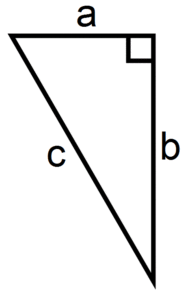
Field distance calculation
Where:
a is the horizontal distance from the center
b is the vertical distance downfield
c is the total sound travel distance
This is critical because most performers are not aligned on a single axis. Drill design creates diagonal timing offsets constantly.
Why the diagonal matters
A performer at the 30-yard line on the back sideline is not necessarily 160 feet away from the person listening on the front sideline. That 160-foot figure only describes a straight front-to-back distance.
If the listener is positioned somewhere else on the field, the actual distance between the performer and listener may be greater because the sound is traveling diagonally. The correct measurement must account for both the horizontal and vertical separation between the two positions.
That difference can affect the calculated sound-travel delay. At close distances, the difference may be relatively small. Across large field distances and faster tempos, however, even small changes in travel time can become musically relevant when performers are trying to achieve extremely precise ensemble alignment.
This is why the exact listening point matters. The timing relationship between two performers is not determined solely by their yard lines or whether they are on the front or back sideline. It depends on the actual distance between the source of the sound and the listener.
For clean ensemble alignment, that distance can be calculated rather than estimated. Once the horizontal and vertical components are known, the diagonal distance can be determined and used to calculate the corresponding sound-travel delay.
In other words, when analyzing timing across a marching field, where you are listening from matters just as much as where the performer is standing.
Practical application on the field
The relationships behind Cost of Timing are not just theoretical. They can be applied directly to marching band and drum corps rehearsal, arranging, and drill design.
For example, you can use these calculations to design front-to-back timing locks, where performers in different parts of the field intentionally adjust their timing to account for the distance sound must travel. Instead of treating the resulting delay as an unavoidable problem, you can predict it and make deliberate timing decisions.
The same principles can be used to create intentional rhythmic delay effects. By controlling when performers play and where they are positioned, designers can create musical moments where sounds arrive at different times for the audience. The physical distance between performers becomes part of the effect.
You can also use the calculations to build split timing across field sections. Different groups can be given timing adjustments based on their positions, allowing the ensemble to compensate for differences in sound travel and improve perceived alignment from a specific listening location.
This becomes especially useful when coordinating pit and battery entrances across extreme distances. A front ensemble positioned near the front sideline and a battery positioned deep on the field can experience substantial differences in sound travel time. Understanding those differences gives instructors another tool for determining how entrances should be coordinated during rehearsal.
The important distinction is that these calculations do not replace musical judgment. They provide a way to quantify a physical effect that performers and instructors are already experiencing.
Once you understand the relationship between distance, sound travel, tempo, and rhythmic subdivision, you can make timing decisions based on measurable information rather than relying entirely on trial and error.
That makes Cost of Timing a practical tool for rehearsal and design, not simply a theoretical exercise in acoustics.
Why triplets and subdivisions matter more than you think
Different rhythmic subdivisions change how a fixed sound delay is perceived. The physical delay does not change simply because the music uses eighth notes, sixteenth notes, or triplets. What changes is the relationship between that delay and the amount of musical time available between rhythmic events.
Eighth notes provide a useful reference for identifying medium-sized timing differences. When performers are separated across significant field distances, the delay between sound production and sound arrival can become noticeable in relation to the eighth-note pulse.
Sixteenth notes make smaller timing differences more apparent. Because the spaces between rhythmic events are shorter, the same physical delay represents a larger portion of each subdivision. A delay that might seem insignificant during slower or less dense material can become much more noticeable when the ensemble is performing a fast sixteenth-note passage.
Triplets introduce another rhythmic framework. Because the subdivision divides the beat differently, the same sound-travel delay can interact with the rhythmic grid in a different way. Across large field distances, this can create interesting differences in how simultaneous or repeated events are perceived.
This helps explain why certain drill moments can feel "cleaner" or "messier" depending on the combination of tempo, rhythmic subdivision, and performer spacing, even when the performers are technically playing at the correct tempo.
The ensemble may be perfectly synchronized at the moment each performer produces a sound, while the audience hears those sounds at slightly different times because they traveled different distances.
That distinction is important. Technical timing and perceived timing are not always identical.
By considering the rhythmic subdivision alongside field geometry and sound-travel delay, instructors and designers can better understand why certain musical moments respond differently to changes in tempo and spacing. What sounds perfectly aligned from one location may sound slightly staggered from another.
The goal is not to treat every perceived timing difference as a mistake. Sometimes the difference is a natural consequence of physics. Understanding that distinction allows instructors to identify when timing needs to be corrected and when the field itself is contributing to what the audience hears.
Field design implications
Once you understand sound delay, you can begin designing drill and music that intentionally accounts for it. Instead of treating the travel time of sound as a problem that must always be corrected, you can use it as another compositional tool.
A backfield performer can produce a musical event slightly earlier so that the sound arrives at the front ensemble at the intended moment. This can be particularly useful when coordinating a backfield entrance with an important musical impact point near the front of the field.
The same principle can be expanded across multiple sections. An across-field rhythmic canon can use performer placement and carefully timed entrances to create a sequence of sounds that travels across the audience's listening field. Each group contributes at a calculated moment, allowing the physical movement of sound to become part of the musical structure.
You can also create spatially phased accents by combining performer location, timing, and sound travel. Multiple performers can produce related musical events at carefully selected times so that the sounds arrive at the audience in a deliberate sequence or resolve together from a specific listening position.
This requires thinking about timing differently. Traditional ensemble timing focuses primarily on when performers produce their sounds. Spatial timing also considers when those sounds arrive at the listener.
That distinction opens another layer of compositional possibilities. Drill position, musical timing, tempo, and acoustic distance can all work together to shape what the audience experiences.
At that point, you are no longer simply trying to make an ensemble sound perfectly synchronized. You are designing compositional timing around the physical space in which the music is being performed.
The field becomes part of the composition.
Summary
Sound delay on a football field is not simply an error to be corrected. It is a design parameter.
Once you can calculate the relationship between distance, sound travel time, tempo, and rhythmic subdivision, you can use that information to make more informed decisions about both rehearsal and musical design.
You can predict ensemble alignment across distance, giving instructors a better understanding of how performers positioned at different locations on the field will perceive one another.
You can design intentional timing effects, using the physical distance between performers to create musical moments that would not be possible in a conventional stage environment.
You can understand why certain drill feels tight or loose, even when performers are technically playing at the correct tempo. The perceived result can change depending on where performers are positioned and where the audience is listening.
And perhaps most importantly, you can use space as a rhythmic instrument. Field position does not have to be separate from the music. Distance, movement, and sound propagation can all become part of the compositional process.
This changes the way we think about marching ensemble timing. The field is not acoustically neutral, and sound does not appear everywhere at once.
Marching band is not just music performance. It is distributed timing physics in motion.
Now, apply this logic to your performance using a SIMPLE APP! SoundDelay.com calculates all this information for you, and gives you the result in BPM, so it’s very easy to apply! Is your drumline coming in late from the back of the field? Use the calculator to tell them EXACTLY how much to anticipate for their entrance!
About the Author
Patrick Blakley is a percussion educator, author, adjudicator, and entrepreneur specializing in marching percussion and drumline education. He is the creator of DrumPacket.com, DrumlineWarmups.com, DrumAudit.com, DrumsetGrooves.com, and SyracuseDrums.com. His educational materials and performance audio edits through CompetitiveMusic.com are used by hundreds of schools and programs across the United States and beyond. He is the author of Quadratics: The Tenor Drum Equation, The Field Percussion User Manual, and other instructional music books. Read more about him by clicking here!
